The reorder point is the critical inventory threshold at which a new purchase or production order must be placed to avoid a stockout before the replenishment arrives. It is mathematically defined as ROP = (Average Daily Demand × Lead Time in Days) + Safety Stock. This calculation ensures that on-hand inventory is sufficient to cover customer demand during the entire replenishment lead time, accounting for the inherent uncertainty in both demand rates and supplier delivery performance.

Glossary
Reorder Point
The predetermined minimum inventory level that triggers a replenishment order, calculated as the expected demand during the lead time plus the safety stock required to buffer against variability.
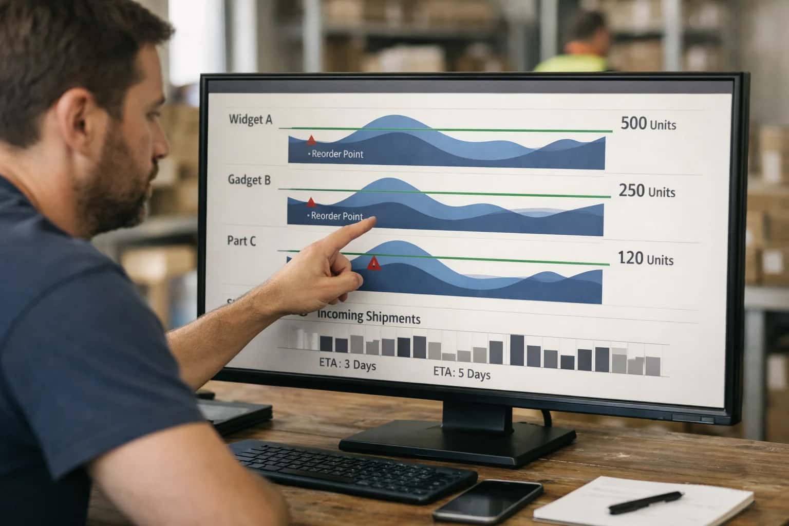
INVENTORY CONTROL FUNDAMENTALS
What is Reorder Point?
The reorder point (ROP) is the predetermined minimum inventory level that triggers a replenishment order, calculated as the expected demand during the lead time plus the safety stock required to buffer against variability.
When inventory position drops to the ROP, a replenishment order for a predetermined quantity—often derived from the Economic Order Quantity (EOQ)—is triggered. In continuous review systems, this check occurs after every transaction, while periodic review systems evaluate inventory against the order-up-to level at fixed intervals. Setting the ROP too low increases the risk of stockouts and lost sales, while setting it too high inflates inventory carrying costs and ties up working capital unnecessarily.
INVENTORY CONTROL FUNDAMENTALS
Key Characteristics of an Effective Reorder Point
A robust reorder point (ROP) is not a static number but a dynamic threshold that balances the cost of stockouts against the cost of holding inventory. The following characteristics define a mathematically sound and operationally resilient ROP.
01
Probabilistic Demand Integration
An effective ROP rejects simple averages in favor of demand distribution modeling. It ingests probabilistic forecasts that quantify uncertainty, typically using a normal or Poisson distribution. The calculation explicitly accounts for the standard deviation of demand during the lead time, not just the mean. This ensures the ROP covers likely demand spikes, not just average consumption, preventing stockouts during predictable volatility.
02
Dynamic Lead Time Sensitivity
The ROP must be directly coupled to supplier lead time variability, not just a static contractual promise. An effective system ingests real-time Predictive Lead Time Analytics to adjust the threshold. If a supplier's delivery variance increases due to geopolitical disruption, the ROP automatically rises to compensate. The formula treats lead time as a stochastic variable with its own mean and standard deviation, preventing a false sense of security from fixed lead time assumptions.
03
Safety Stock Decomposition
A transparent ROP explicitly separates cycle stock (demand during average lead time) from safety stock (buffer against variability). The safety stock component is calculated using a desired Cycle Service Level (CSL) or Fill Rate target. For a 99% CSL, the safety stock factor (Z-score) is 2.33. This decomposition allows finance teams to audit the cost of service-level policies directly against the working capital tied up in the buffer.
04
Multi-Echelon Visibility
An isolated ROP creates the Bullwhip Effect. An effective ROP is calculated with visibility into upstream echelons. It considers the inventory position at the supplying warehouse, not just the local stock. In a Guaranteed Service Model (GSM), the ROP is set to cover the guaranteed processing time of the upstream node. This holistic view prevents redundant safety stock accumulation across the network and optimizes total system inventory.
05
Continuous Recalculation Engine
A static ROP decays in relevance immediately. An effective system employs a rolling horizon or event-driven architecture that recalculates the threshold daily or intra-daily. It ingests fresh demand sensing signals from point-of-sale data and real-time inventory positions. This dynamic adjustment captures demand shifts, promotions, and supply disruptions instantly, ensuring the ROP is always optimized for the current operational reality rather than a stale historical snapshot.
06
Exception-Based Alerting
The ROP system should not require constant human monitoring. It must feature exception-based management triggers that fire when the inventory position breaches the ROP or when the ROP itself changes beyond a defined tolerance. Alerts should differentiate between a standard replenishment signal and a critical stockout risk. This allows planners to focus on resolving high-impact anomalies rather than manually reviewing thousands of SKUs that are behaving within expected parameters.
REORDER POINT ESSENTIALS
Frequently Asked Questions
Clear, technically precise answers to the most common questions about calculating and applying reorder points in multi-echelon inventory optimization.
A reorder point (ROP) is the predetermined minimum inventory level that triggers a replenishment order, calculated as the expected demand during the lead time plus the safety stock required to buffer against variability. When the inventory position—the sum of on-hand stock and on-order quantities minus backorders—drops to or below this threshold, the system automatically generates a new purchase or production order. The core mechanism is expressed as ROP = (d × LT) + SS, where d is the average demand per period, LT is the lead time in periods, and SS is the safety stock. This ensures that new stock arrives just as the last unit of safety stock is consumed, preventing stockouts while minimizing excess holding costs. In a multi-echelon inventory optimization context, the reorder point at each node must account for upstream variability and the service level targets of downstream nodes.
Enabling Efficiency, Speed & Accuracy
Intelligent Analysis, Decision & Execution
We build AI systems for teams that need search across company data, workflow automation across tools, or AI features inside products and internal software.
Talk to Us
Search across company data
Give teams answers from docs, tickets, runbooks, and product data with sources and permissions.
Useful when people spend too long searching or get different answers from different systems.
Enterprise searchRAGPermissions
Read more
Automate internal workflows
Use AI to route work, draft outputs, trigger actions, and keep approvals and logs in place.
Useful when repetitive work moves across multiple tools and teams.
AI agentsWorkflow automationGovernance
Read more
Add AI to products and internal tools
Build assistants, guided actions, or decision support into the software your team or customers already use.
Useful when AI needs to be part of the product, not a separate tool.
AI integrationDecision supportModel routing
Read moreINVENTORY CONTROL POLICY COMPARISON
Reorder Point vs. Order-Up-To Level
Structural and operational differences between the two primary inventory replenishment triggers used in continuous and periodic review systems.
| Feature | Reorder Point (ROP) | Order-Up-To Level (OUTL) | Hybrid (s,S) Policy |
|---|---|---|---|
Review Type | Continuous | Periodic | Continuous |
Trigger Mechanism | Inventory position hits ROP | Review interval elapses | Inventory position ≤ s |
Order Quantity | Fixed (Q) | Variable (S - current position) | Variable (S - current position) |
Primary Cost Driver | Holding + ordering cost trade-off | Holding + shortage cost trade-off | Holding + ordering + shortage cost trade-off |
Safety Stock Protection | Lead time demand variability only | Lead time + review period demand variability | Lead time demand variability only |
Best For | Stable demand, high-volume SKUs | Low-volume, irregular demand patterns | Erratic demand, high-value items |
Computational Complexity | Low | Moderate | High |
Risk of Stockout Between Reviews | Low (continuous monitoring) | Higher (blind between intervals) | Low (continuous monitoring) |

About the author
Prasad Kumkar
CEO & MD, Inference Systems
Prasad Kumkar is the CEO & MD of Inference Systems and writes about AI systems architecture, LLM infrastructure, model serving, evaluation, and production deployment. Over 5+ years, he has worked across computer vision models, L5 autonomous vehicle systems, and LLM research, with a focus on taking complex AI ideas into real-world engineering systems.
His work and writing cover AI systems, large language models, AI agents, multimodal systems, autonomous systems, inference optimization, RAG, evaluation, and production AI engineering.
LinkedIn
Limited slotsGet a Free AI Consultation
Partnered with leading AI, data, and software stack.





How We Work
Custom AI workflows for your Business
One-fit-all AI don't work for modern businesses. At Inferensys, we aim to understand your business & custom requirements; which we use to define most efficient agentic workflows, the data, and the tools for your business.
01
Review the use case
We understand the task, the users, and where AI can actually help.
Read more02
Pick the right approach
We define what needs search, automation, or product integration.
Read more03
Build the first useful version
We implement the part that proves the value first.
Read more04
Improve from there
We add the checks and visibility needed to keep it useful.
Read moreThe first call is a practical review of your use case and the right next step.
Talk to Us