Guide

How to Build a Production RFML Pipeline for Signal Identification

A developer guide to constructing a scalable MLOps pipeline for RF signal classification, covering data ingestion, feature extraction, model training, and deployment with continuous monitoring.

Get in touch Learn more

Data scientist building training data pipeline on laptop, data preprocessing visible, technical workspace.

RFML PIPELINE

Introduction

This guide details the construction of a robust, end-to-end machine learning pipeline for Radio Frequency Machine Learning (RFML). You will learn to transform raw RF signals into a deployed, monitored system capable of identifying unique emitters.

A production RFML pipeline automates the journey from raw IQ data to actionable intelligence. It encompasses data ingestion, feature extraction, model training, and scalable deployment. Unlike experimental notebooks, this pipeline ensures reproducibility, continuous training, and performance monitoring, which are critical for applications in wireless security and electronic warfare. The core challenge is handling the high-dimensional, complex nature of RF signals within a reliable MLOps framework.

You will implement this using tools like PyTorch or TensorFlow for model development and Kubeflow or MLflow for orchestration. Key steps include designing a streaming data architecture, implementing model versioning, and establishing feedback loops for model retraining. This systematic approach is essential for moving from proof-of-concept to a system that operates reliably in dynamic, real-world RF environments, such as those monitored for spectrum awareness.

PRODUCTION RFML PIPELINE

Key Concepts

Building a robust RFML pipeline requires mastering these core components, from raw signal ingestion to a monitored, deployed model.

Signal Preprocessing & Feature Extraction

Raw IQ data is noisy and high-dimensional. Preprocessing cleans the signal (filtering, normalization) while feature extraction reduces dimensionality and highlights discriminative patterns. Common techniques include:

Generating spectrograms or cyclostationary profiles
Calculating higher-order statistics (cumulants)
Extracting transient features from signal onsets This step transforms raw waveforms into a format suitable for machine learning, directly impacting model accuracy and training efficiency.

Model Architecture & Training

RF signal identification is a specialized classification task. Effective architectures must capture both temporal and spectral patterns.

Convolutional Neural Networks (CNNs) excel at learning from spectrogram images.
Recurrent Networks (RNNs/LSTMs) model temporal sequences in IQ data.
Hybrid CNN-RNN models combine both strengths. Training requires domain-specific data augmentation (adding noise, frequency shifts) to improve robustness. Use frameworks like PyTorch or TensorFlow with Weights & Biases for experiment tracking.

MLOps & Pipeline Orchestration

A production pipeline automates the model lifecycle. Key components include:

Data Versioning (DVC) to track datasets and preprocessing code.
Experiment Tracking (MLflow) to log parameters, metrics, and artifacts.
Pipeline Orchestration (Kubeflow, Apache Airflow) to chain data ingestion, training, and validation steps.
Model Registry to stage, version, and promote models for deployment. This infrastructure enables reproducible experiments, continuous training, and collaboration across engineering and data science teams.

Model Serving & Inference

Deploying trained models for real-time or batch inference requires a scalable serving layer.

REST/gRPC APIs (using TensorFlow Serving or TorchServe) provide standard interfaces.
Edge Deployment on devices like NVIDIA Jetson requires model optimization via pruning and quantization.
Streaming Inference architectures (Apache Kafka, Flink) process continuous IQ data streams. Implement A/B testing and shadow deployment to validate new models against production traffic before full cutover.

Performance Monitoring & Drift Detection

Production models degrade. Continuous monitoring is non-negotiable.

Data Drift: Monitor statistical properties of incoming IQ signals versus the training set.
Concept Drift: Track changes in the relationship between features and predictions (e.g., new emitter types).
Model Performance: Log inference latency, throughput, and business metrics. Set up automated alerts to trigger model retraining or pipeline review when thresholds are breached, ensuring system reliability.

Related Guides & Next Steps

This pipeline integrates several specialized domains. For deeper dives, explore our related guides:

Data Strategy: Learn to plan and manage RF datasets in How to Design a Data Strategy for RF Fingerprinting Model Development.
Edge Deployment: Implement low-latency systems with How to Implement Real-Time Signal Classification at the Edge.
System Security: Architect defenses against active threats with How to Build a System for Detecting RF Spoofing and Jamming Attacks.

FOUNDATION

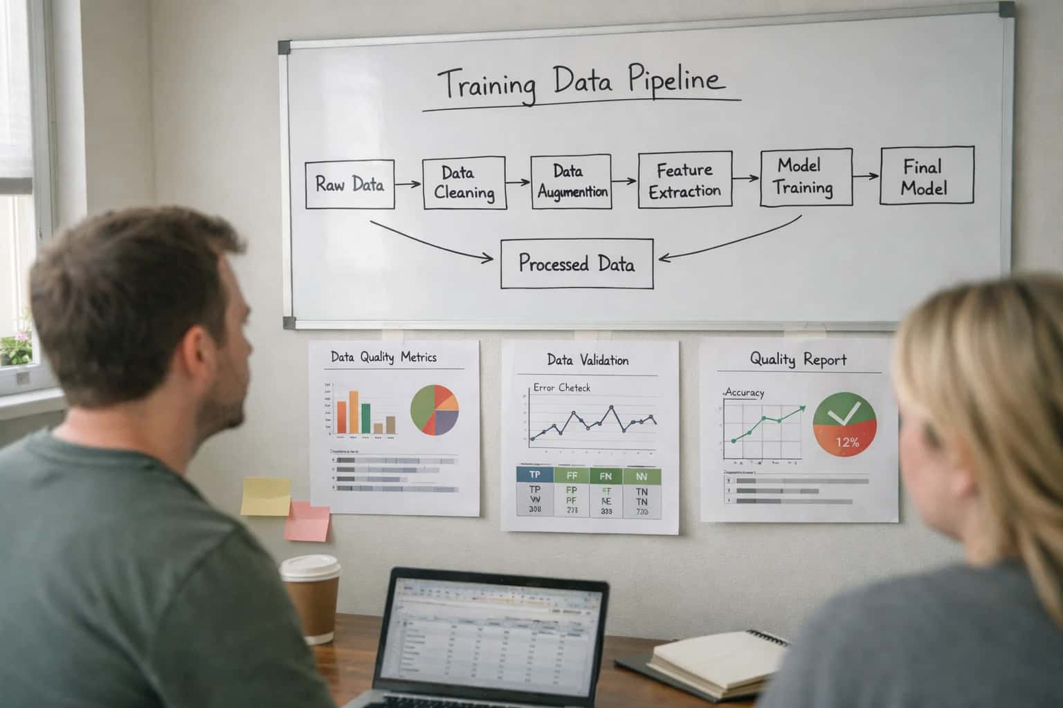
Step 1: Design the Pipeline Architecture

A robust, scalable architecture is the non-negotiable foundation of any production RFML system. This step defines the data flow, component responsibilities, and integration points that determine long-term success.

A production RFML pipeline is a directed acyclic graph (DAG) of specialized stages. You must design for data lineage, reproducibility, and scalability from the outset. Core stages include: raw IQ data ingestion from SDRs or files, preprocessing (filtering, normalization), feature extraction (generating spectrograms or cyclostationary features), model training/inference, and results storage/visualization. Each stage should be a containerized, stateless service for independent scaling, managed by an orchestrator like Kubeflow or Apache Airflow.

Key architectural decisions involve choosing between a batch processing paradigm for model retraining and a streaming paradigm (e.g., using Apache Kafka or Apache Flink) for real-time identification. Your design must also specify the model registry (MLflow), feature store, and monitoring hooks for data drift and model performance. This blueprint directly enables the continuous training and deployment cycles detailed in our guide on MLOps for agentic systems.

PIPELINE ORCHESTRATION

MLOps Framework Comparison

This table compares core MLOps frameworks for managing the lifecycle of an RFML pipeline, from experiment tracking to model deployment and monitoring.

Feature / Capability	MLflow	Kubeflow	Custom Airflow + DVC
Experiment & Model Registry
Native Pipeline Orchestration
Hyperparameter Tuning Integration	MLflow Tracking	Katib	Manual / Optuna
RF-Specific Data Versioning	via Plugins	via Artifacts	via DVC Core
Kubernetes-Native Deployment	MLflow Models		Manual YAML
Real-Time Inference Monitoring	MLflow Model Registry	KFServing + Prometheus	Custom Dashboard
IQ Data Lineage Tracking	Limited	via Metadata	via DVC Pipelines
On-Prem / Air-Gapped Support

MLOPS DEPLOYMENT

Step 5: Deploy Models with Kubeflow or MLflow

This step transitions your trained RFML model from an experiment to a reliable, scalable service. You will package the model, its dependencies, and the inference logic for production.

Model deployment is the process of serving your trained RF fingerprinting classifier as an API for real-time inference. Kubeflow orchestrates this on Kubernetes, managing scaling, health checks, and rollouts, ideal for high-throughput systems. MLflow simplifies deployment by packaging models, code, and a Conda environment into a single artifact, which can be served locally or on a cloud platform. Both frameworks handle versioning, so you can roll back if a new model underperforms, a core concept in MLOps for agentic systems.

To deploy, first log your PyTorch model and its preprocessing pipeline in MLflow. Then, build a Docker container with the MLflow model server or define a Kubeflow Pipeline component. For RF signals, ensure your deployment includes the same feature extraction steps used in training. Finally, integrate monitoring to track prediction latency, throughput, and potential model drift over time, which is critical for maintaining system reliability in dynamic RF environments.

Enabling Efficiency, Speed & Accuracy

Intelligent Analysis, Decision & Execution

We build AI systems for teams that need search across company data, workflow automation across tools, or AI features inside products and internal software.

Talk to Us

Search across company data

Give teams answers from docs, tickets, runbooks, and product data with sources and permissions.

Useful when people spend too long searching or get different answers from different systems.

Enterprise searchRAGPermissions

Automate internal workflows

Use AI to route work, draft outputs, trigger actions, and keep approvals and logs in place.

Useful when repetitive work moves across multiple tools and teams.

AI agentsWorkflow automationGovernance

Add AI to products and internal tools

Build assistants, guided actions, or decision support into the software your team or customers already use.

Useful when AI needs to be part of the product, not a separate tool.

AI integrationDecision supportModel routing

TROUBLESHOOTING

Common Mistakes

Building a production RFML pipeline involves unique pitfalls from data to deployment. This section addresses the most frequent technical errors that derail projects, providing clear solutions to keep your signal identification system robust.

This is the classic overfitting to hardware artifacts problem. Your model learns features specific to your lab's single USRP or antenna, not the intrinsic transmitter fingerprint.

Solution: Implement a rigorous data strategy.

Collect data from multiple SDRs and antennas to force the model to learn hardware-invariant features.
Use synthetic data augmentation that mimics channel effects (multipath, Doppler) and receiver imperfections (phase noise, IQ imbalance). Tools like MATLAB or GNU Radio can generate this.
Apply domain adaptation techniques during training to align feature distributions between your source (lab) and target (field) data domains.

Failing to plan for hardware variance during data collection is the most common root cause of deployment failure.

About the author

Prasad Kumkar

CEO & MD, Inference Systems

Prasad Kumkar is the CEO & MD of Inference Systems and writes about AI systems architecture, LLM infrastructure, model serving, evaluation, and production deployment. Over 5+ years, he has worked across computer vision models, L5 autonomous vehicle systems, and LLM research, with a focus on taking complex AI ideas into real-world engineering systems.

His work and writing cover AI systems, large language models, AI agents, multimodal systems, autonomous systems, inference optimization, RAG, evaluation, and production AI engineering.

Limited slotsGet a Free AI Consultation

How We Work

Custom AI workflows for your Business

One-fit-all AI don't work for modern businesses. At Inferensys, we aim to understand your business & custom requirements; which we use to define most efficient agentic workflows, the data, and the tools for your business.