Demand sensing is a forecasting methodology that leverages real-time, downstream data signals—such as daily point-of-sale (POS) transactions, warehouse withdrawals, and short-term weather patterns—to refine near-term demand predictions. Unlike traditional statistical models that rely solely on historical shipment data, demand sensing reduces latency by capturing immediate consumption signals, typically improving forecast accuracy for a 1- to 4-week horizon.

Glossary
Demand Sensing
A forecasting technique that uses real-time, short-term data signals—such as point-of-sale transactions and weather—to refine near-term demand predictions and reduce latency in the supply chain.
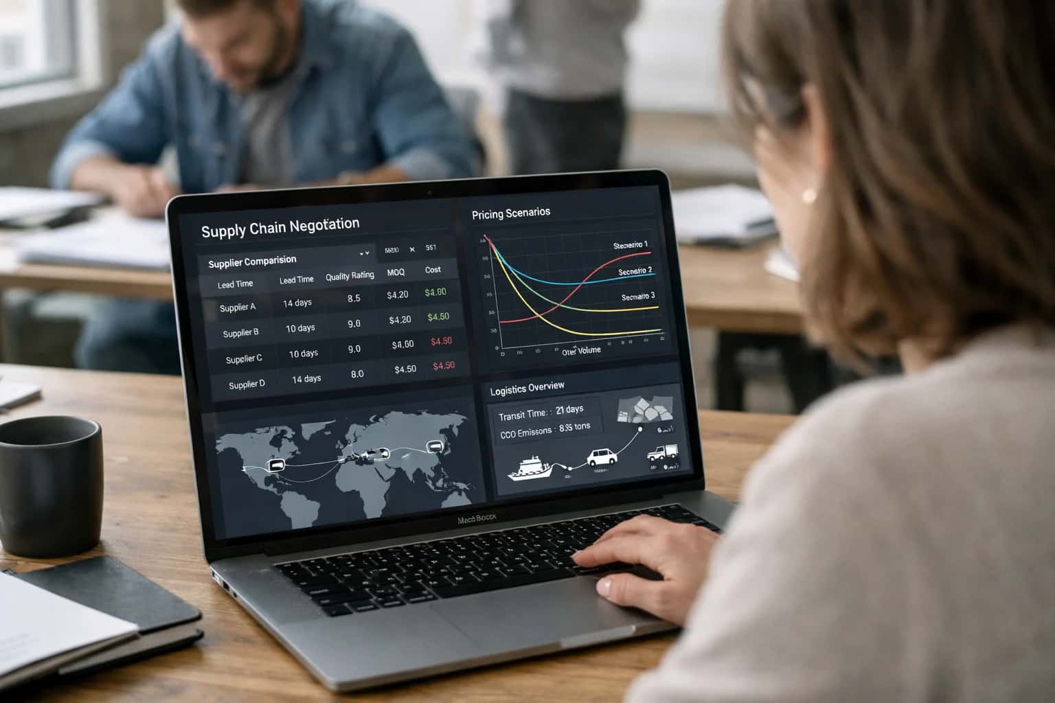
REAL-TIME FORECASTING
What is Demand Sensing?
A short-horizon forecasting technique that translates real-time demand signals into actionable replenishment decisions.
The technique employs machine learning algorithms to automatically correlate disparate short-cycle data streams, detecting demand shifts that lagging indicators miss. By integrating external regressors like local events or competitor pricing, demand sensing enables a demand-driven supply chain, allowing inventory planners to dynamically adjust safety stock and replenishment parameters to prevent stockouts without inflating upstream volatility.
NEAR-TERM FORECASTING ARCHITECTURE
Key Characteristics of Demand Sensing
Demand sensing distinguishes itself from traditional forecasting through its reliance on high-velocity, short-horizon data signals. The following characteristics define its technical implementation and operational value in a modern supply chain.
01
Short-Term Horizon Focus
Demand sensing operates on a rolling horizon of 1 to 14 days, contrasting sharply with traditional statistical models that project weeks or months into the future. This narrow window allows the model to capture immediate market shifts. The objective is not long-range planning but the precise refinement of near-term operational signals, such as tomorrow's distribution requirements. By limiting the prediction window, the system minimizes the accumulation of forecast error inherent in long-range projections and reacts exclusively to current, actionable data.
02
Real-Time Signal Ingestion
The core differentiator is the ingestion of latency-sensitive, downstream data that traditional models ignore. This includes daily Point-of-Sale (POS) transactions, hourly e-commerce clickstreams, and warehouse withdrawal data. The architecture connects directly to operational data stores to process structured and semi-structured feeds. By analyzing what is actually selling right now—rather than historical shipment averages—the system detects demand shifts as they happen, bypassing the information lag that creates the bullwhip effect upstream.
03
Exogenous Variable Integration
Demand sensing models systematically incorporate external regressors to explain short-term variance that historical patterns alone cannot capture. Key inputs include localized weather forecasts, social media sentiment analysis, and competitor pricing intelligence. For example, a sudden temperature drop can be correlated with an immediate spike in specific SKU sales. The model learns the causal relationship between these external events and demand lift, allowing it to adjust predictions before the effect fully materializes in the order stream.
04
Automated Pattern Recognition
Unlike manually adjusted forecasts, demand sensing employs machine learning algorithms to autonomously detect complex, non-linear patterns in high-dimensional data. Techniques range from gradient boosting machines to recurrent neural networks. The system automatically identifies subtle correlations—such as the interaction between a holiday, a price promotion, and a weather event—that would be impossible for a human planner to calculate manually. This automation ensures that the forecast adapts continuously without requiring constant human intervention to tweak baseline predictions.
05
Downstream Data Proximity
The architecture prioritizes data sources closest to the end consumer to bypass the bullwhip effect. By ingesting retailer POS data or syndicated scanner data, the model observes true consumer take-away rather than distorted upstream orders. This creates a demand signal that is independent of inventory policies or order batching at intermediate nodes. The result is a highly accurate, un-distorted view of consumption that allows manufacturers to synchronize production schedules directly with actual market pull, reducing the need for excessive safety stock.
06
Latency Reduction in S&OP
Demand sensing bridges the gap between rigid Sales & Operations Planning (S&OP) cycles and daily execution. Traditional monthly S&OP processes cannot react to a mid-month demand shock. Demand sensing provides a continuous, automated feedback loop that generates a revised daily forecast. This allows supply chain teams to make intra-week adjustments to inventory deployment and production sequencing. The result is a dramatic reduction in the latency between a market signal and the operational response, moving the organization closer to a real-time enterprise model.
DEMAND SENSING EXPLAINED
Frequently Asked Questions
Clear, technical answers to the most common questions about translating real-time signals into near-term demand predictions for supply chain optimization.
Demand sensing is a forecasting technique that leverages real-time, short-term data signals to refine near-term demand predictions, typically within a 1- to 6-week horizon. Unlike traditional forecasting that relies on aggregated historical shipment data, demand sensing ingests high-velocity downstream data such as point-of-sale (POS) transactions, warehouse withdrawals, and retailer inventory levels. The process works by applying machine learning algorithms—often gradient boosting or recurrent neural networks—to detect demand patterns and shifts that classical time-series models miss. By mathematically weighting recent signals more heavily than older history, the model reduces forecast latency and adapts to sudden market changes. This creates a closed feedback loop where actual consumption data continuously corrects the statistical forecast, enabling supply chain planners to make more accurate replenishment decisions and reduce the bullwhip effect upstream.
METHODOLOGY COMPARISON
Demand Sensing vs. Traditional Forecasting
A technical comparison of short-horizon demand sensing against classical statistical forecasting methods across key operational dimensions.
| Dimension | Demand Sensing | Traditional Forecasting | Hybrid Approach |
|---|---|---|---|
Data Latency | Real-time (sub-hourly) | Batch (daily/weekly) | Mixed-frequency ingestion |
Primary Data Signals | POS, clicks, weather, social | Historical shipments, orders | Both historical and real-time |
Forecast Horizon | 1 day to 6 weeks | 4 weeks to 18 months | 1 week to 6 months |
Model Architecture | Pattern recognition, ML | Statistical (ARIMA, ETS) | Ensemble of both |
Handles Intermittent Demand | |||
Bullwhip Effect Mitigation | |||
Granularity | SKU-store-hour | SKU-DC-week | SKU-store-day |
Response to Demand Shocks | < 4 hours | 1-2 planning cycles | < 24 hours |
Enabling Efficiency, Speed & Accuracy
Intelligent Analysis, Decision & Execution
We build AI systems for teams that need search across company data, workflow automation across tools, or AI features inside products and internal software.
Talk to Us
Search across company data
Give teams answers from docs, tickets, runbooks, and product data with sources and permissions.
Useful when people spend too long searching or get different answers from different systems.
Enterprise searchRAGPermissions
Read more
Automate internal workflows
Use AI to route work, draft outputs, trigger actions, and keep approvals and logs in place.
Useful when repetitive work moves across multiple tools and teams.
AI agentsWorkflow automationGovernance
Read more
Add AI to products and internal tools
Build assistants, guided actions, or decision support into the software your team or customers already use.
Useful when AI needs to be part of the product, not a separate tool.
AI integrationDecision supportModel routing
Read more
About the author
Prasad Kumkar
CEO & MD, Inference Systems
Prasad Kumkar is the CEO & MD of Inference Systems and writes about AI systems architecture, LLM infrastructure, model serving, evaluation, and production deployment. Over 5+ years, he has worked across computer vision models, L5 autonomous vehicle systems, and LLM research, with a focus on taking complex AI ideas into real-world engineering systems.
His work and writing cover AI systems, large language models, AI agents, multimodal systems, autonomous systems, inference optimization, RAG, evaluation, and production AI engineering.
LinkedIn
Limited slotsGet a Free AI Consultation
Partnered with leading AI, data, and software stack.





How We Work
Custom AI workflows for your Business
One-fit-all AI don't work for modern businesses. At Inferensys, we aim to understand your business & custom requirements; which we use to define most efficient agentic workflows, the data, and the tools for your business.
01
Review the use case
We understand the task, the users, and where AI can actually help.
Read more02
Pick the right approach
We define what needs search, automation, or product integration.
Read more03
Build the first useful version
We implement the part that proves the value first.
Read more04
Improve from there
We add the checks and visibility needed to keep it useful.
Read moreThe first call is a practical review of your use case and the right next step.
Talk to Us