A Jacobian matrix is a first-order partial derivative matrix that linearly maps the instantaneous velocities of a system's inputs to the velocities of its outputs. In robotics, it directly relates joint velocities to the resulting end-effector velocity in Cartesian space. This linear approximation is crucial for inverse kinematics, force control, and analyzing system singularities where the mapping becomes degenerate and controllability is lost.

Glossary
Jacobian Matrix
In robotics, a Jacobian matrix is a mathematical construct that linearly relates the velocity of a robot's end-effector in Cartesian space to the velocities of its individual joints.
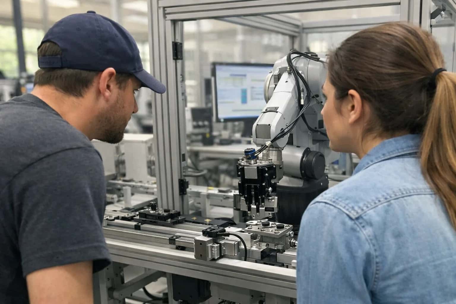
ROBOTICS & CONTROL
What is a Jacobian Matrix?
A fundamental mathematical tool in robotics, computer vision, and machine learning that quantifies the relationship between input changes and output changes in a multivariable system.
Beyond kinematics, the Jacobian is central to backpropagation in neural networks, where it propagates error gradients through layers. In optimization, it defines the local landscape for algorithms like Gauss-Newton. For Vision-Language-Action models, the Jacobian enables differentiable planning, allowing gradient-based optimization of action sequences with respect to high-level visual and language goals by quantifying how small motor adjustments affect task success.
ROBOTIC KINEMATICS
Core Properties of the Jacobian Matrix
The Jacobian matrix is a fundamental tool in robotics that linearly maps joint velocities to end-effector velocity. Its properties are critical for analyzing robot motion, singularities, and force transmission.
01
Linear Velocity Transformation
The primary function of the Jacobian J(q) is to provide a first-order, linear approximation of the relationship between joint velocities and end-effector velocity. For a robot with n joints and an m-dimensional task space, the mapping is defined as:
v = J(q) * q̇
- v is the m x 1 twist vector (linear and angular velocity) of the end-effector.
- q̇ is the n x 1 vector of joint velocities.
- J(q) is the m x n Jacobian matrix, whose elements are functions of the current joint configuration q.
This linear relationship is valid for instantaneous motion and is derived from the robot's forward kinematics.
02
Singular Configurations
A singularity occurs when the Jacobian matrix loses full rank, meaning it becomes rank-deficient. At these joint configurations q_s:
- The robot loses one or more degrees of freedom in Cartesian space.
- Certain end-effector velocities become impossible to achieve.
- The inverse mapping from desired velocity to required joint velocity becomes ill-posed (infinite solutions or no solution).
Singularities are classified:
- Boundary Singularities: Occur at the workspace limits.
- Internal Singularities: Occur within the workspace due to kinematic alignment (e.g., a fully extended elbow in a serial manipulator).
Identifying singularities is essential for robust motion planning and control.
03
Force-Torque Duality
Through the principle of virtual work, the Jacobian provides a dual relationship between forces in joint space and Cartesian space. If F is a wrench (force-torque vector) applied at the end-effector, the equivalent joint torques τ required to resist it are:
τ = J(q)^T * F
- This property is fundamental for force control and impedance control.
- It allows the robot to modulate its stiffness in Cartesian space by adjusting joint torques.
- The transpose of the Jacobian maps forces from the task space back to the actuator space, enabling tasks like assembly and pushing.
04
Manipulability Ellipsoid
The manipulability ellipsoid is a geometric visualization of the robot's velocity capabilities derived from the Jacobian. It is defined by the matrix J * J^T.
- The eigenvectors of J * J^T define the principal axes of the ellipsoid in Cartesian space.
- The lengths of the axes (the square roots of the eigenvalues) represent the maximum achievable end-effector velocity in those directions for a unit norm of joint velocity.
- A spherical ellipsoid indicates isotropic manipulability—equal ease of movement in all directions.
- A flattened ellipsoid indicates the robot moves much more easily in certain directions than others.
The volume of this ellipsoid is a common metric for quantifying a configuration's dexterity.
05
Analytical vs. Geometric Derivation
The Jacobian can be computed using two primary methods:
1. Analytical (Velocity Propagation) Method:
- Uses the chain rule to differentiate the forward kinematic equations directly.
- Results in a symbolic matrix that is a function of joint variables.
- Well-suited for computational efficiency in control loops.
2. Geometric (Vector Cross Product) Method:
- Constructs the Jacobian column-by-column based on the geometry of the manipulator.
- For a revolute joint i, column i is: [ z_i x (p_ee - p_i) ; z_i ] where z_i is the joint axis and p are position vectors.
- For a prismatic joint, column i is: [ z_i ; 0 ].
- This method provides physical intuition about how each joint contributes to end-effector motion.
06
Role in Inverse Kinematics & Control
The Jacobian is central to many real-time kinematic solutions and control laws:
- Jacobian Transpose Control: A simple, computationally efficient algorithm for force control or motion using Δq = α J^T * e, where e is a Cartesian error.
- Jacobian Pseudoinverse: Used to solve for joint velocities from desired end-effector velocity: q̇ = J⁺ * v, where J⁺ is the Moore-Penrose pseudoinverse. This handles redundant manipulators (n > m).
- Damped Least Squares (DLS): A singularity-robust method using q̇ = J^T (J J^T + λ²I)⁻¹ v, which trades off accuracy near singularities for finite joint velocities.
- Resolved-Rate Motion Control: A standard technique where the desired Cartesian trajectory's derivative is used as v in the equation q̇ = J⁻¹ * v (or its pseudoinverse variant).
TASK AND MOTION PLANNING
How the Jacobian Matrix Works in Robotics
A core mathematical tool for relating robot joint motion to end-effector movement, enabling velocity control, force analysis, and singularity detection.
In robotics, the Jacobian matrix is a first-order partial derivative matrix that linearly maps the velocity of a robot's joints to the velocity (both linear and angular) of its end-effector in Cartesian space. This relationship, expressed as v = J(q) * q_dot, is fundamental for velocity control, inverse kinematics solvers, and analyzing manipulability. The matrix's structure depends entirely on the robot's kinematic chain and current joint configuration q.
The Jacobian is critically used for force transformation via its transpose, mapping end-effector forces to equivalent joint torques. Its determinant reveals kinematic singularities, where the robot loses a degree of freedom. In motion planning and trajectory optimization, the Jacobian enables the computation of Cartesian paths from joint-space commands and is essential for resolved-rate motion control and impedance control algorithms.
THE JACOBIAN MATRIX
Practical Applications in Robotics
The Jacobian matrix is a foundational mathematical tool in robotics that linearly maps joint velocities to end-effector velocities. Its applications are critical for real-time control, force manipulation, and motion analysis.
01
Velocity Control & Motion Planning
The primary application of the Jacobian matrix is to compute the required joint velocities to achieve a desired end-effector velocity. This is essential for real-time trajectory tracking and path following.
- Inverse Velocity Kinematics: Given a desired Cartesian velocity (\dot{x}), the required joint velocities (\dot{q}) are approximated by (\dot{q} = J(q)^{\dagger} \dot{x}), where (J(q)^{\dagger}) is the pseudoinverse of the Jacobian.
- Singularity Avoidance: Near kinematic singularities, the Jacobian becomes ill-conditioned, causing unrealistically high joint velocities. Algorithms use the manipulability measure (the determinant of (J J^T)) to detect and avoid these configurations.
- Example: For a robotic arm painting a car door, the Jacobian continuously maps the desired paint sprayer tip velocity to the motor speeds of each joint.
02
Static Force & Torque Mapping
Through the duality of kinematics and statics, the transpose of the Jacobian matrix maps forces applied at the end-effector to the equivalent torques required at the joints. This is governed by the principle of virtual work.
- Force Transformation: The relationship is (\tau = J(q)^T F), where (F) is a force/torque vector at the end-effector and (\tau) is the vector of joint torques.
- Key Applications:
- Impedance Control: Regulating the interaction force between the robot and its environment.
- Assistive Robotics: Enabling exoskeletons or cobots to apply specific assistive forces.
- Grasping Analysis: Determining the joint torques needed to exert a desired gripping force without crushing an object.
03
Singularity Analysis & Dexterity
The Jacobian is the key to analyzing a robot's kinematic performance. Its properties determine where the robot loses or gains mobility.
- Manipulability Ellipsoid: The eigenvectors and eigenvalues of (J(q)J(q)^T) define an ellipsoid in Cartesian space. The principal axes show the directions of maximum and minimum end-effector velocity for a unit joint velocity sphere.
- Condition Number: The ratio of the largest to smallest singular value of the Jacobian. A high condition number indicates an ill-conditioned configuration near a singularity, where motion in some directions is very limited.
- Application: This analysis is used in robot design to optimize link lengths and joint ranges, and in task placement to ensure a robot operates in its most dexterous workspace.
04
Inverse Kinematics (IK) Solvers
While analytical IK provides closed-form solutions, numerical IK methods rely heavily on the Jacobian for iterative convergence to a desired end-effector pose.
- Newton-Raphson Method: A common iterative approach. The pose error (e = x_d - x) is reduced by updating joint angles: (q_{new} = q_{old} + J(q_{old})^{\dagger} e).
- Damped Least-Squares (DLS): A more robust variant that solves (\dot{q} = (J^T J + \lambda^2 I)^{-1} J^T \dot{x}). The damping factor (\lambda) prevents instability near singularities.
- Use Case: Essential for robots with redundant degrees of freedom (e.g., 7-DoF arms) or complex geometries where analytical solutions don't exist, enabling them to reach around obstacles.
05
Redundancy Resolution & Null-Space Control
For kinematically redundant robots (more joints than task-space dimensions), the Jacobian defines a null space. This allows secondary objectives to be achieved without affecting the primary end-effector task.
- Null-Space Projection: The general solution for joint velocities is (\dot{q} = J^{\dagger} \dot{x} + (I - J^{\dagger}J) \dot{q}_0). The term ((I - J^{\dagger}J)) projects any vector (\dot{q}_0) into the null space.
- Secondary Objectives: (\dot{q}_0) can be chosen to:
- Maximize manipulability.
- Avoid joint limits.
- Minimize power consumption.
- Perform a secondary task (e.g., pointing a camera).
- Example: A 7-DoF surgical robot can maintain precise tool tip positioning (primary task) while reconfiguring its elbow to avoid a physical obstacle (secondary null-space task).
06
Dynamics & Control Law Formulation
The Jacobian appears in the derivation of advanced model-based control laws, connecting kinematics to the equations of motion.
- Operational Space Dynamics: Newton-Euler equations are transformed from joint space to task (operational) space using the Jacobian. The dynamic equation becomes (\Lambda(q) \ddot{x} + \mu(q, \dot{q}) + p(q) = F), where (\Lambda(q) = (J M^{-1} J^T)^{-1}) is the operational space inertia matrix.
- Applications in Control:
- Computed Torque Control: Uses the full dynamic model for precise tracking.
- Hybrid Force/Position Control: Decouples control into force-controlled and position-controlled directions in task space, defined via the Jacobian.
- Foundation for Simulation: The Jacobian is critical in physics engines for computing constraint forces and simulating contact dynamics between a robot and its environment.
KINEMATIC MAPPINGS
Jacobian vs. Related Kinematic Concepts
A comparison of the Jacobian matrix to other fundamental mathematical objects in robotics kinematics and planning, highlighting their distinct purposes and outputs.
| Feature / Concept | Jacobian Matrix | Forward Kinematics | Inverse Kinematics (IK) |
|---|---|---|---|
Primary Function | Maps joint velocities to end-effector velocity (differential kinematics) | Maps joint angles to end-effector pose | Maps desired end-effector pose to required joint angles |
Core Mathematical Object | Matrix (first-order partial derivatives) | Non-linear vector function | Non-linear, often ill-posed, inverse function |
Typical Output | End-effector linear & angular velocity (twist) | End-effector position & orientation (pose) | Set of joint angle solutions |
Dimensionality | 6 x N (for N joints in 3D space) | 6-dimensional pose vector | N-dimensional joint angle vector |
Linearity of Relationship | Linear approximation at a given configuration | Inherently non-linear | Inherently non-linear |
Key Use Case in Planning | Velocity control, singularity analysis, force transformation | State validation, goal specification | Goal pose satisfaction for motion primitives |
Computational Complexity (per query) | O(N), analytic or numeric | O(N), closed-form | Iterative (O(kN)) or closed-form if available |
Uniqueness of Solution | Unique mapping for a given configuration (matrix is defined) | Unique pose for a given joint set | Often multiple or infinite solutions (kinematic redundancy) |
JACOBIAN MATRIX
Frequently Asked Questions
Essential questions and answers about the Jacobian matrix, a foundational mathematical tool in robotics and machine learning for relating changes in joint space to changes in task space.
In robotics, a Jacobian matrix is a mathematical construct that provides a linear approximation of the relationship between the velocity of a robot's joints and the resulting velocity (both linear and angular) of its end-effector in Cartesian space. It is a function of the robot's current joint configuration. Formally, if q is the vector of joint angles and x is the pose of the end-effector, the Jacobian J(q) satisfies the equation ẋ = J(q)q̇, where q̇ is the vector of joint velocities and ẋ is the resulting end-effector twist. This matrix is central to velocity kinematics, inverse kinematics solvers, singularity analysis, and force transformation.
Enabling Efficiency, Speed & Accuracy
Intelligent Analysis, Decision & Execution
We build AI systems for teams that need search across company data, workflow automation across tools, or AI features inside products and internal software.
Talk to Us
Search across company data
Give teams answers from docs, tickets, runbooks, and product data with sources and permissions.
Useful when people spend too long searching or get different answers from different systems.
Enterprise searchRAGPermissions
Read more
Automate internal workflows
Use AI to route work, draft outputs, trigger actions, and keep approvals and logs in place.
Useful when repetitive work moves across multiple tools and teams.
AI agentsWorkflow automationGovernance
Read more
Add AI to products and internal tools
Build assistants, guided actions, or decision support into the software your team or customers already use.
Useful when AI needs to be part of the product, not a separate tool.
AI integrationDecision supportModel routing
Read more
About the author
Prasad Kumkar
CEO & MD, Inference Systems
Prasad Kumkar is the CEO & MD of Inference Systems and writes about AI systems architecture, LLM infrastructure, model serving, evaluation, and production deployment. Over 5+ years, he has worked across computer vision models, L5 autonomous vehicle systems, and LLM research, with a focus on taking complex AI ideas into real-world engineering systems.
His work and writing cover AI systems, large language models, AI agents, multimodal systems, autonomous systems, inference optimization, RAG, evaluation, and production AI engineering.
LinkedIn
Limited slotsGet a Free AI Consultation
Partnered with leading AI, data, and software stack.





How We Work
Custom AI workflows for your Business
One-fit-all AI don't work for modern businesses. At Inferensys, we aim to understand your business & custom requirements; which we use to define most efficient agentic workflows, the data, and the tools for your business.
01
Review the use case
We understand the task, the users, and where AI can actually help.
Read more02
Pick the right approach
We define what needs search, automation, or product integration.
Read more03
Build the first useful version
We implement the part that proves the value first.
Read more04
Improve from there
We add the checks and visibility needed to keep it useful.
Read moreThe first call is a practical review of your use case and the right next step.
Talk to Us