Model partitioning is the technique of splitting a neural network's computational graph across multiple processing units or edge nodes to execute layers in parallel when a single device lacks sufficient memory or compute capacity. This is essential for deploying large models on resource-constrained factory-floor hardware, enabling pipeline parallelism where sequential layers are distributed, or tensor parallelism where individual operations are sharded.

Glossary
Model Partitioning
Model partitioning is the technique of splitting a neural network's computational graph across multiple processing units or edge nodes to execute layers in parallel when a single device lacks sufficient memory or compute capacity.
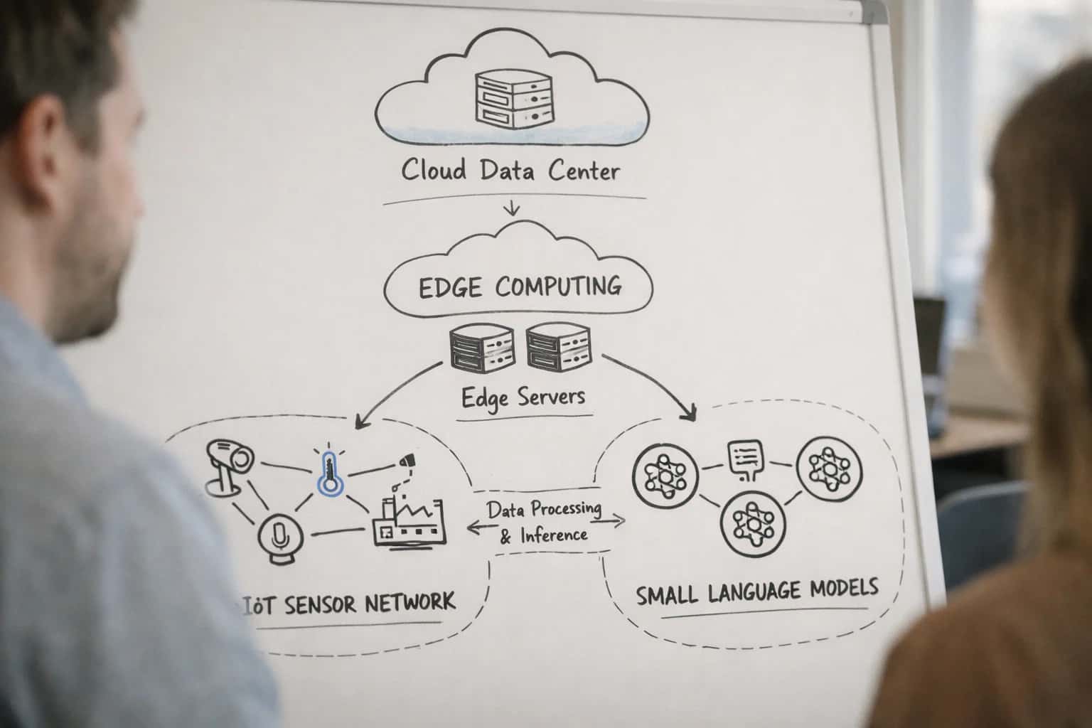
DISTRIBUTED INFERENCE
What is Model Partitioning?
Model partitioning is the strategic decomposition of a neural network's computational graph into distinct segments for parallel execution across multiple processing units or edge nodes, overcoming the memory and compute limitations of a single device.
Effective partitioning requires analyzing the model's dataflow graph to identify optimal split points that minimize inter-device communication overhead while maximizing hardware utilization. Frameworks like heterogeneous compute architectures and neural network compilers automate this process, mapping subgraphs to the most efficient silicon—CPUs, GPUs, or NPUs—within a distributed edge cluster to achieve deterministic, low-latency inference.
DISTRIBUTED INFERENCE ARCHITECTURES
Key Characteristics of Model Partitioning
Model partitioning is a fundamental technique for deploying large neural networks on resource-constrained edge hardware. By splitting a computational graph across multiple accelerators or nodes, inference becomes feasible where a single device lacks sufficient memory or compute capacity.
01
Pipeline Parallelism
Partitions a model by layer depth, assigning contiguous groups of layers to different devices. Each device processes its assigned layers and passes intermediate activations to the next device in the pipeline.
- Micro-batching splits input data into smaller chunks to keep all devices busy concurrently, reducing idle time between pipeline stages
- Commonly used for large language models and deep vision transformers where layer count exceeds single-GPU memory
- Introduces a bubble overhead at pipeline start and end, which can be minimized with scheduling optimizations like GPipe or PipeDream
- Example: A 96-layer transformer can be split across 4 GPUs, each handling 24 layers sequentially
3-5x
Throughput Improvement
02
Tensor Parallelism
Splits individual weight matrices within a single layer across multiple devices, parallelizing the matrix multiplication operations themselves. Each device holds a shard of the weight tensor and computes a partial result.
- Requires high-bandwidth interconnects like NVLink or InfiniBand due to frequent all-reduce communication between devices after every forward and backward pass
- Ideal for layers with massive parameter counts that exceed the memory of a single accelerator
- Often combined with pipeline parallelism in a hybrid 3D parallelism strategy for training and inference of trillion-parameter models
- Example: A single attention head's QKV projection matrix can be split column-wise across 4 GPUs, with each computing a portion of the output
< 1 ms
All-Reduce Latency Target
03
Expert Parallelism
Leverages the Mixture of Experts (MoE) architecture, where different sub-networks called experts are placed on separate devices. A gating mechanism routes each input token to only a subset of experts, activating only a fraction of the total parameters per inference.
- Dramatically increases total model capacity without proportionally increasing compute cost, as only top-k experts are activated per token
- Introduces load balancing challenges to prevent expert starvation or overload, requiring auxiliary loss functions during training
- Well-suited for edge deployments where expert shards can be distributed across a cluster of lower-power nodes
- Example: Mixtral 8x7B uses 8 experts with 2 active per token, achieving 47B-parameter quality at 13B-parameter inference cost
8-64
Typical Expert Count
04
Data Parallelism with Model Replicas
Replicates the entire model across multiple devices, with each replica processing a different subset of the input batch. Gradients are synchronized across replicas after each backward pass during training.
- During inference, this pattern enables horizontal scaling to increase throughput by serving multiple inference requests concurrently on separate replicas
- Does not reduce the memory footprint of a single model instance, so it cannot solve the problem of a model being too large for one device
- Often combined with dynamic batching to maximize utilization of each replica's compute capacity
- Example: A quality inspection model replicated across 10 edge nodes, each processing images from a different camera on the production line
Near-linear
Throughput Scaling
05
Sequence Parallelism
Distributes the long sequence dimension of input data across multiple devices, complementing tensor parallelism for transformer models processing extended contexts. Each device computes attention and feed-forward operations on its assigned sequence segment.
- Critical for models handling long context windows exceeding 8K tokens, where activation memory from the attention mechanism dominates total memory consumption
- Uses ring-style communication patterns to share key-value pairs between devices during the attention computation
- Reduces peak activation memory proportionally to the number of devices, enabling inference on sequences that would otherwise cause out-of-memory errors
- Example: A 32K-token context can be split across 4 GPUs, each processing 8K tokens with cross-device attention communication
4x
Max Context Length Extension
06
Edge-Cloud Hybrid Partitioning
Splits a model between an edge device and a cloud server, executing initial layers locally for feature extraction and offloading computationally intensive later layers to the cloud. This balances latency, privacy, and compute constraints.
- Early exit branches can be inserted at the partition point, allowing the edge to make fast predictions for simple inputs without invoking the cloud
- Reduces data transmission by sending compact intermediate representations rather than raw sensor data, preserving bandwidth and enhancing privacy
- Requires careful bottleneck design at the partition point to minimize the size of transmitted tensors while preserving sufficient information for accurate downstream processing
- Example: A defect detection model runs the first 3 convolutional layers on a smart camera, sending feature maps to a factory-edge server for final classification layers
10-100x
Bandwidth Reduction vs Raw Data
Enabling Efficiency, Speed & Accuracy
Intelligent Analysis, Decision & Execution
We build AI systems for teams that need search across company data, workflow automation across tools, or AI features inside products and internal software.
Talk to Us
Search across company data
Give teams answers from docs, tickets, runbooks, and product data with sources and permissions.
Useful when people spend too long searching or get different answers from different systems.
Enterprise searchRAGPermissions
Read more
Automate internal workflows
Use AI to route work, draft outputs, trigger actions, and keep approvals and logs in place.
Useful when repetitive work moves across multiple tools and teams.
AI agentsWorkflow automationGovernance
Read more
Add AI to products and internal tools
Build assistants, guided actions, or decision support into the software your team or customers already use.
Useful when AI needs to be part of the product, not a separate tool.
AI integrationDecision supportModel routing
Read moreMODEL PARTITIONING
Frequently Asked Questions
Clear, technically precise answers to the most common questions about splitting neural network computational graphs across edge hardware for factory-floor deployment.
Model partitioning is the technique of splitting a neural network's computational graph into distinct subgraphs and distributing them across multiple processing units or edge nodes for parallel execution. This strategy is employed when a single device—such as an industrial PC or smart camera—lacks sufficient memory or compute capacity to run the entire model. The process involves analyzing the model's directed acyclic graph to identify optimal split points based on tensor shapes, data dependencies, and inter-layer communication costs. Partitioning can occur along several dimensions: layer-wise (vertical splitting where early layers run on one device and later layers on another), tensor-parallel (horizontal splitting where individual weight matrices are sharded across devices), or pipeline-parallel (where micro-batches are streamed through a chain of devices, each responsible for a contiguous segment of layers). In manufacturing edge deployments, a common pattern partitions a vision model so that convolutional feature extractors execute on an NPU-accelerated smart camera while the classification head runs on a nearby industrial PC, minimizing data transfer while respecting hardware constraints.

About the author
Prasad Kumkar
CEO & MD, Inference Systems
Prasad Kumkar is the CEO & MD of Inference Systems and writes about AI systems architecture, LLM infrastructure, model serving, evaluation, and production deployment. Over 5+ years, he has worked across computer vision models, L5 autonomous vehicle systems, and LLM research, with a focus on taking complex AI ideas into real-world engineering systems.
His work and writing cover AI systems, large language models, AI agents, multimodal systems, autonomous systems, inference optimization, RAG, evaluation, and production AI engineering.
LinkedIn
Limited slotsGet a Free AI Consultation
Partnered with leading AI, data, and software stack.





How We Work
Custom AI workflows for your Business
One-fit-all AI don't work for modern businesses. At Inferensys, we aim to understand your business & custom requirements; which we use to define most efficient agentic workflows, the data, and the tools for your business.
01
Review the use case
We understand the task, the users, and where AI can actually help.
Read more02
Pick the right approach
We define what needs search, automation, or product integration.
Read more03
Build the first useful version
We implement the part that proves the value first.
Read more04
Improve from there
We add the checks and visibility needed to keep it useful.
Read moreThe first call is a practical review of your use case and the right next step.
Talk to Us