Trajectory Optimization

Trajectory optimization problems are fundamentally defined by the system dynamics—the differential equations governing state evolution—and a set of hard and soft constraints. These constraints ensure the solution is physically realizable and safe.

• State Constraints: Limit the permissible values of the system's state variables (e.g., joint angles, velocity, position).
• Control Constraints: Bound the admissible control inputs (e.g., torque, thrust, voltage).
• Path Constraints: Impose conditions that must hold throughout the entire trajectory (e.g., obstacle avoidance, staying within a corridor).
• Terminal Constraints: Specify conditions that must be met at the trajectory's endpoint (e.g., precise final position and zero velocity).

Violating these constraints renders a trajectory infeasible, making their accurate modeling the first step in any optimization formulation.

The objective of trajectory optimization is to minimize a scalar cost function, which quantifies the quality or desirability of a trajectory. This function encodes the trade-offs between competing goals like speed, energy efficiency, and smoothness.

Common cost formulations include:

• Bolza Form: A standard form combining a terminal cost (Mayer term) and an integrated running cost (Lagrange term): J = φ(x(t_f), t_f) + ∫ L(x(t), u(t), t) dt.
• Quadratic Cost: Often used for linear systems (LQR problems), penalizing deviations from a reference and control effort: J = ∫ (x^T Q x + u^T R u) dt.
• Minimum Time: A special case where the cost is simply J = t_f, the final time.
• Minimum Control Effort: Penalizes the magnitude of control inputs to conserve energy.

The choice of cost function directly steers the optimizer's search, making it a critical design parameter that aligns the mathematical solution with the practical objective.

Trajectory optimization is rooted in optimal control theory, which provides the mathematical conditions for optimality. The most fundamental principle is the Pontryagin's Minimum Principle (PMP), which provides necessary conditions for an optimal control trajectory.

PMP introduces costate variables (adjoints) λ(t) and defines the Hamiltonian: H(x, u, λ, t) = L(x, u, t) + λ^T f(x, u, t), where f describes the system dynamics. For an optimal trajectory (x*(t), u*(t)), there exists a costate trajectory λ*(t) such that:

• State Equation: dx/dt = ∂H/∂λ
• Costate Equation: dλ/dt = -∂H/∂x
• Minimization Condition: H(x*(t), u*(t), λ*(t), t) ≤ H(x*(t), v, λ*(t), t) for all admissible controls v.

These conditions transform the optimization problem into a two-point boundary value problem, which can be solved numerically.

Numerical approaches to solving trajectory optimization problems are broadly categorized into direct and indirect methods, differing in how they handle the optimality conditions.

Direct Methods (Transcription):

• Discretize the state and control trajectories first, converting the infinite-dimensional problem into a finite-dimensional Nonlinear Programming (NLP) problem.
• Examples: Direct Collocation, Direct Shooting, Pseudospectral Methods.
• Pros: Easier to handle complex constraints; more robust to initial guesses.
• Cons: Large-scale NLP problems can be computationally intensive.

Indirect Methods:

• First apply the necessary conditions from Pontryagin's Minimum Principle to derive the optimality system (a boundary value problem).
• Then discretize and solve this system.
• Pros: Can yield highly accurate solutions that satisfy optimality conditions precisely.
• Cons: Sensitive to initial guesses for costates; difficult to handle path constraints.

In modern practice, direct methods are more commonly used due to their robustness and flexibility.

Trajectory optimization is a cornerstone for planning and control in physical autonomous systems, enabling precise, efficient, and safe motion.

Key Applications:

• Robot Manipulators: Planning smooth, collision-free paths for robotic arms in manufacturing (e.g., welding, assembly) and logistics (e.g., pick-and-place).
• Autonomous Vehicles: Computing lane-change maneuvers, merging trajectories, and parking paths that obey vehicle dynamics and traffic rules.
• Aerospace & Drones: Planning fuel-optimal ascent trajectories for rockets or agile flight paths for quadrotors through cluttered environments.
• Legged Locomotion: Generating stable walking and running gaits for humanoid and quadruped robots by optimizing contact forces and body motions.

These applications typically use frameworks like Model Predictive Control (MPC), which repeatedly solves a finite-horizon trajectory optimization problem online, using new sensor data to update the plan and account for disturbances.

Trajectory optimization and model-based reinforcement learning (MBRL) are deeply connected paradigms for sequential decision-making. Both aim to find an optimal sequence of actions, but their assumptions and methodologies differ.

Trajectory Optimization assumes a known, accurate model of the system dynamics and cost function. It performs planning by solving the optimization problem directly using the model.

Model-Based RL often uses trajectory optimization as a subroutine for planning within a learned model. The agent:

1. Learns an approximate dynamics model from interaction data.
2. Uses trajectory optimization (e.g., via Model Predictive Control) to plan actions within this learned model.
3. Executes the plan, collects new data, and refines the model.

This hybrid approach, sometimes called Model-Based RL with Planning, combines the sample efficiency of trajectory optimization with RL's ability to adapt to unknown environments. Algorithms like PILCO and PETS exemplify this synergy.

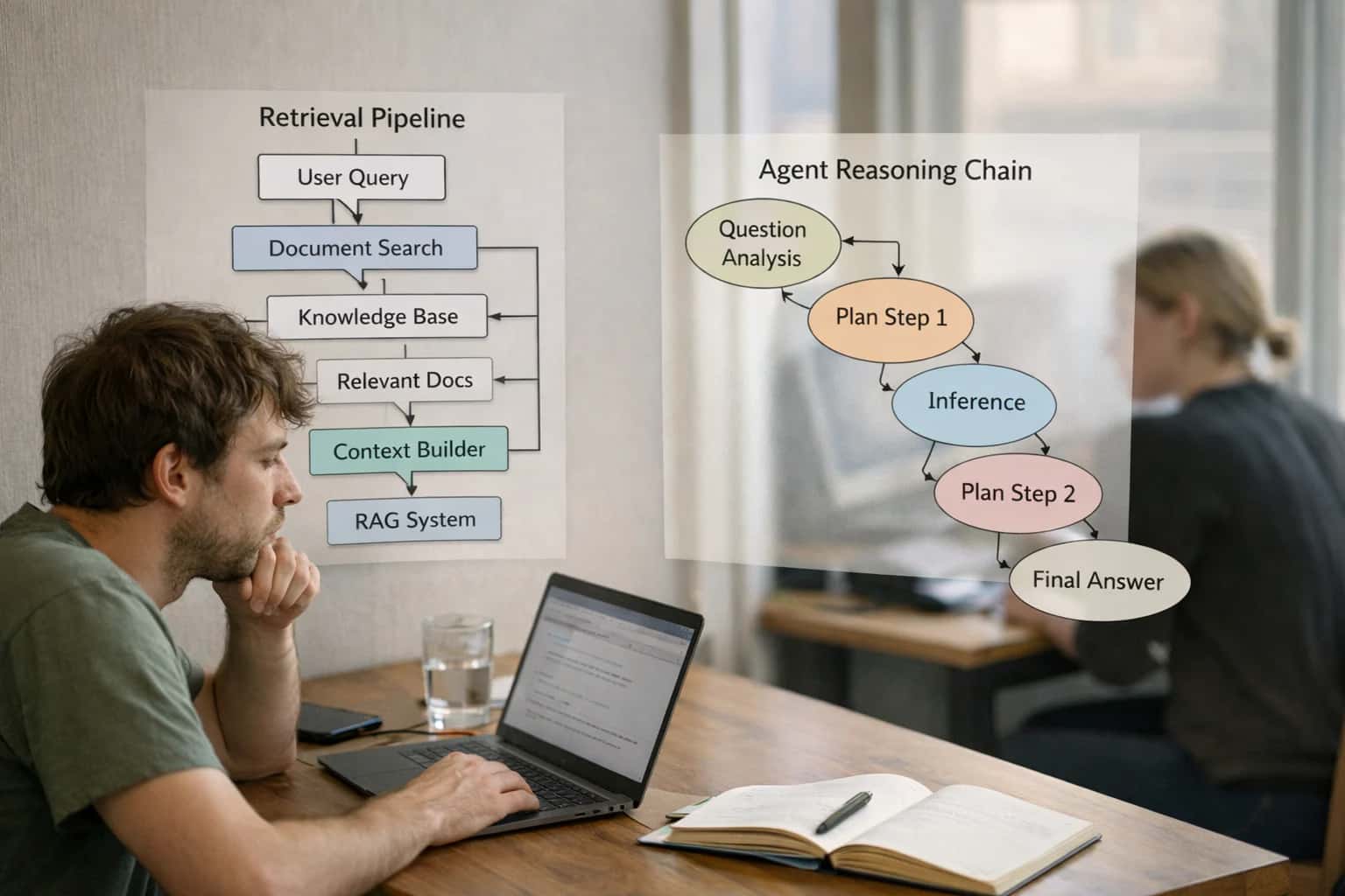
In agentic cognitive architectures, trajectory optimization principles apply to planning sequences of tool calls and API executions. The 'state' is the digital context, and 'control inputs' are discrete actions like database queries or code execution.

• Corrective Action Planning: When an agent detects an error, it re-optimizes its future action sequence (trajectory) to reach the corrected goal.
• Multi-Step Reasoning: Framing a chain-of-thought as a trajectory through a 'reasoning space' to be optimized for correctness and efficiency.
• Resource-Constrained Execution: Planning action sequences that minimize cost (e.g., LLM token usage) or latency within a fault-tolerant system.

Optimizes time-varying setpoints for complex industrial processes to maximize yield, quality, and efficiency while adhering to safety limits. This often involves non-linear system dynamics and path constraints.

• Chemical Reactors: Controlling temperature and feed rates to maximize product output and purity.
• Batch Processing: Optimizing the time-profile of operations in pharmaceutical manufacturing.
• Robotic Welding/Additive Manufacturing: Computing optimal toolhead speed and power trajectories for consistent material deposition.

A real-time, receding horizon control strategy that solves a finite-horizon trajectory optimization problem at each time step. It uses an explicit model of the system to predict future states, computes an optimal sequence of control inputs, but only implements the first step before re-solving with new measurements. This makes it highly robust to model inaccuracies and disturbances.

• Core Mechanism: Solves a constrained optimization online.
• Key Feature: Feedback through re-planning.
• Primary Use: Robotics, process control, autonomous vehicles.

The foundational mathematical framework for sequential decision-making under uncertainty. An MDP formalizes a problem with states, actions, transition probabilities, and rewards. Trajectory optimization in stochastic environments is essentially the search for an optimal policy within an MDP framework.

• States & Actions: Define the decision space.
• Transition Function: Models system dynamics (can be stochastic).
• Objective: Maximize cumulative expected reward.

A machine learning paradigm where an agent learns a policy through trial-and-error interaction with an environment to maximize cumulative reward. Many RL algorithms, especially in continuous control, are solving a trajectory optimization problem without an explicit dynamics model. Model-based RL explicitly learns a dynamics model for planning.

• Connection: RL seeks optimal trajectories via learning.
• Model-Based vs. Model-Free: Spectrum of approaches.
• Example Algorithms: PPO, SAC, DDPG.

The computational problem of finding a feasible path for a robot from a start to a goal configuration while avoiding obstacles. Trajectory optimization adds the dimension of time and dynamics, turning a geometric path into a time-parameterized trajectory that satisfies kinodynamic constraints (e.g., velocity, acceleration, torque limits).

• Path vs. Trajectory: A path is geometric; a trajectory includes timing.
• Sampling-Based Planners: RRT*, PRM find initial paths for optimization.
• Application: Robotic arm manipulation, autonomous navigation.

The broader mathematical field concerned with finding a control law for a dynamical system over time to minimize a cost functional. Trajectory optimization is a central problem in optimal control. Classical solutions include Pontryagin's Maximum Principle (which provides necessary conditions for optimality) and Dynamic Programming (which solves via the Hamilton-Jacobi-Bellman equation).

• Theoretical Foundation: Provides necessary conditions for optimality.
• Direct vs. Indirect Methods: Two main numerical approaches.
• Historical Context: Rooted in calculus of variations.

A sample-efficient, global optimization strategy for expensive black-box functions. It is used for trajectory optimization when the cost function is complex, non-convex, or lacks an analytic gradient. It builds a probabilistic surrogate model (like a Gaussian Process) to guide the search for optimal parameters.

• Use Case: Optimizing hyperparameters of a policy or controller.
• Key Strength: Balances exploration and exploitation.
• Application: Tuning robotic gaits, controller parameters.