Model drift detection is the operational safeguard that continuously compares the statistical distribution of live inference data against a reference baseline established during training. In RFML systems, this process monitors for data drift—shifts in the input IQ sample distribution—and concept drift, where the fundamental relationship between signal features and their correct labels changes due to new hardware or interference patterns. The mechanism computes divergence metrics such as the Kullback-Leibler divergence or Maximum Mean Discrepancy between windowed production data and the training set to trigger alerts before silent failure occurs.

Glossary
Model Drift Detection
The continuous monitoring process that identifies when a deployed RFML model's statistical properties diverge from its training baseline due to changes in the electromagnetic environment.
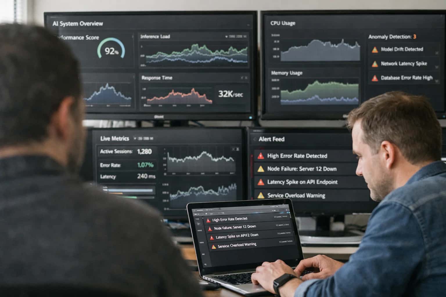
PRODUCTION MONITORING
What is Model Drift Detection?
Model drift detection is the continuous monitoring process that identifies when a deployed RFML model's statistical properties diverge from its training baseline due to changes in the electromagnetic environment.
Effective detection architectures log prediction confidence scores and input embeddings to a monitoring store, enabling automated statistical hypothesis tests against the baseline. When a drift alarm fires, the system can invoke a digital twin for root-cause analysis or trigger a retraining pipeline. This is critical for specific emitter identification and automatic modulation classification models, where an unrecognized transmitter or a new channel condition can catastrophically degrade accuracy without explicit error signals.
MODEL DRIFT DETECTION
Types of Drift in RFML
Model drift in Radio Frequency Machine Learning refers to the degradation of a deployed model's predictive performance due to a statistical mismatch between its static training environment and the dynamic, evolving electromagnetic operating environment. Effective drift detection is critical for maintaining the reliability of cognitive radio, emitter identification, and spectrum awareness systems.
01
Covariate Shift (Feature Drift)
The most common form of drift, occurring when the statistical distribution of the input IQ data P(X) changes, while the conditional distribution of the label given the input P(Y|X) remains constant. In RFML, this manifests as a shift in the signal-to-noise ratio (SNR), the appearance of new interference types, or a change in the channel's delay spread.
- Example: A modulation classifier trained on high-SNR, line-of-sight (LOS) signals fails when deployed in a low-SNR, non-line-of-sight (NLOS) multipath environment.
- Detection Method: Use a two-sample statistical test like Maximum Mean Discrepancy (MMD) on the latent feature embeddings of a reference and a production data window.
P(X)
Distribution that changes
02
Prior Probability Shift (Label Drift)
A change in the distribution of the target classes P(Y) without a change in the likelihood P(X|Y). In an RF spectrum monitoring context, this happens when a previously rare emitter type suddenly becomes dominant, or a new operational mode is introduced.
- Example: A peacetime spectrum monitoring model encounters a sudden surge of frequency-hopping spread spectrum (FHSS) signals during a military exercise, a class that was severely underrepresented in the training set.
- Detection Method: Monitor the marginal distribution of the model's softmax output probabilities using a drift detector like the Kolmogorov-Smirnov (KS) test on the prediction confidence scores.
P(Y)
Distribution that changes
03
Concept Drift (Posterior Shift)
The most severe form of drift, where the fundamental relationship between the input and the target changes, meaning P(Y|X) is no longer stable. The same IQ sample now corresponds to a different true class. This often indicates a change in the physical hardware or transmission protocol.
- Example: A specific emitter identification (SEI) model trained to fingerprint a particular radar's power amplifier non-linearity begins to fail after the adversary replaces the amplifier hardware, altering the unique fingerprint.
- Detection Method: Requires ground-truth labels in production, making it the hardest to detect online. Performance metrics like accuracy or F1-score are calculated on a delayed labeled sample set and compared against a baseline.
P(Y|X)
Distribution that changes
04
Virtual Drift (Temporal Domain Shift)
A drift pattern specific to time-series RF data where the statistical properties of the channel evolve over time, even if the emitter behavior is static. This is driven by physical phenomena like Doppler spread from moving reflectors or channel aging in a mobile environment.
- Example: An autoencoder-based neural receiver trained for a static pedestrian channel experiences catastrophic decoding failure when the user enters a high-speed vehicle, drastically changing the Doppler profile.
- Detection Method: Track the reconstruction error of a variational autoencoder (VAE) trained on nominal channel conditions. A sustained increase in the reconstruction loss signals a departure from the learned temporal dynamics.
Doppler
Key physical driver
05
Adversarial Drift
A deliberate, malicious form of concept drift where an attacker introduces carefully crafted adversarial perturbations to the input signal to force misclassification. Unlike natural drift, these perturbations are designed to be imperceptible to traditional statistical monitoring while maximizing model error.
- Example: An adversary transmits a waveform with a subtle, optimized perturbation layer that causes an automatic modulation classifier (AMC) to confuse a QPSK signal with a 16-QAM signal, evading detection.
- Detection Method: Use a separate outlier detector based on the local intrinsic dimensionality (LID) of the model's hidden layer activations, which is sensitive to the adversarial subspace.
LID
Detection metric
06
Data Quality Drift (Silent Failure)
A non-statistical form of drift caused by a failure in the signal processing pipeline rather than the environment. This includes sensor miscalibration, IQ imbalance, local oscillator (LO) leakage, or a change in the digital-to-analog converter's (DAC) sampling rate.
- Example: A temperature-induced DC offset in the receiver's analog front-end introduces a constant tone at the center frequency, corrupting all downstream IQ samples and causing the model to see a non-existent carrier.
- Detection Method: Implement data validation checks on raw IQ statistics (mean, variance, kurtosis) and spectral flatness before inference. A schema violation triggers an alert before the corrupted data reaches the model.
IQ Stats
Validation check
MODEL DRIFT DETECTION
Frequently Asked Questions
Addressing the most critical operational questions about identifying and mitigating statistical divergence in deployed radio frequency machine learning systems.
Model drift detection is the continuous monitoring process that identifies when a deployed RFML model's statistical properties diverge from its training baseline due to changes in the electromagnetic environment. In radio frequency applications, drift manifests when the joint probability distribution P(X, y) of input signals and their labels shifts from the distribution observed during training. This divergence degrades classification accuracy for tasks like automatic modulation classification and specific emitter identification. Detection mechanisms typically monitor the model's output softmax confidence distributions, feature embedding drift in latent space, or raw IQ sample statistics. Unlike traditional software monitoring, RF drift detection must account for physically-induced distribution shifts—such as new interference sources, seasonal foliage changes affecting multipath, or hardware aging in transmitter front-ends—that are invisible to standard application performance monitoring tools.
Enabling Efficiency, Speed & Accuracy
Intelligent Analysis, Decision & Execution
We build AI systems for teams that need search across company data, workflow automation across tools, or AI features inside products and internal software.
Talk to Us
Search across company data
Give teams answers from docs, tickets, runbooks, and product data with sources and permissions.
Useful when people spend too long searching or get different answers from different systems.
Enterprise searchRAGPermissions
Read more
Automate internal workflows
Use AI to route work, draft outputs, trigger actions, and keep approvals and logs in place.
Useful when repetitive work moves across multiple tools and teams.
AI agentsWorkflow automationGovernance
Read more
Add AI to products and internal tools
Build assistants, guided actions, or decision support into the software your team or customers already use.
Useful when AI needs to be part of the product, not a separate tool.
AI integrationDecision supportModel routing
Read more
About the author
Prasad Kumkar
CEO & MD, Inference Systems
Prasad Kumkar is the CEO & MD of Inference Systems and writes about AI systems architecture, LLM infrastructure, model serving, evaluation, and production deployment. Over 5+ years, he has worked across computer vision models, L5 autonomous vehicle systems, and LLM research, with a focus on taking complex AI ideas into real-world engineering systems.
His work and writing cover AI systems, large language models, AI agents, multimodal systems, autonomous systems, inference optimization, RAG, evaluation, and production AI engineering.
LinkedIn
Limited slotsGet a Free AI Consultation
Partnered with leading AI, data, and software stack.





How We Work
Custom AI workflows for your Business
One-fit-all AI don't work for modern businesses. At Inferensys, we aim to understand your business & custom requirements; which we use to define most efficient agentic workflows, the data, and the tools for your business.
01
Review the use case
We understand the task, the users, and where AI can actually help.
Read more02
Pick the right approach
We define what needs search, automation, or product integration.
Read more03
Build the first useful version
We implement the part that proves the value first.
Read more04
Improve from there
We add the checks and visibility needed to keep it useful.
Read moreThe first call is a practical review of your use case and the right next step.
Talk to Us